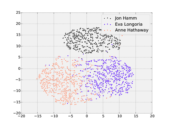
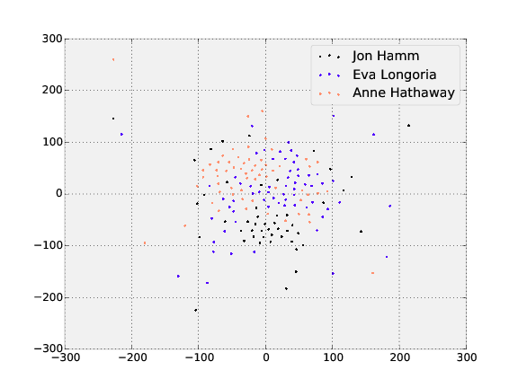
Visualizing representations with t-SNE

t-SNE is a dimensionality reduction technique that can be used to visualize the 128-dimensional features OpenFace produces. The following shows the visualization of the three people in the training and testing dataset with the most images.

Training

Testing

These can be generated with the following commands from the root openface directory.

1. Create raw image directory.

Create a directory for a subset of raw images that you want to visualize with TSNE. Make images from different people are in different subdirectories. The names of the labels or images do not matter, and each person can have a different amount of images. The images should be formatted as jpg or png and have a lowercase extension.

$ tree data/mydataset-subset/raw
person-1
├── image-1.jpg
├── image-2.png
...
└── image-p.png

...

person-m
├── image-1.png
├── image-2.jpg
...
└── image-q.png

2. Preprocess the raw images

Change 8 to however many separate processes you want to run: for N in {1..8}; do ./util/align-dlib.py <path-to-raw-data> align outerEyesAndNose <path-to-aligned-data> --size 96 & done.

If failed alignment attempts causes your directory to have too few images, you can use our utility script ./util/prune-dataset.py to deletes directories with less than a specified number of images.

3. Generate Representations

./batch-represent/main.lua -outDir <feature-directory> -data <path-to-aligned-data> creates reps.csv and labels.csv in <feature-directory>.

4. Generate TSNE visualization

Generate the t-SNE visualization with ./util/tsne.py <feature-directory> --names <name 1> ... <name n>, where name i corresponds to label i from the left-most column in labels.csv. This creates tsne.pdf in <feature-directory>.

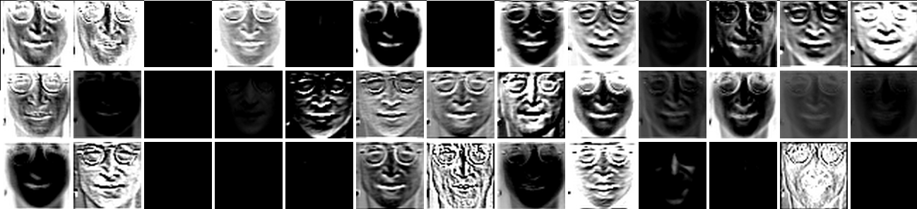
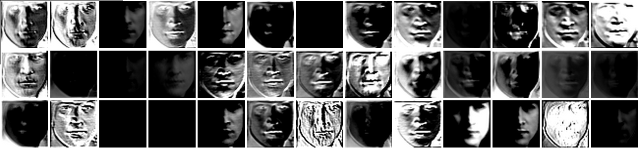
Visualizing layer outputs

Visualizing the output feature maps of each layer is sometimes helpful to understand what features the network has learned to extract. With faces, the locations of the eyes, nose, and mouth should play an important role.

demos/vis-outputs.lua outputs the feature maps from an aligned image. The following shows the first 39 filters of the first convolutional layer on two images of John Lennon.